• Camera Models
  • Projection (3D → 2D)
• Appendix:
  • 1. Forward Projection (3D → 2D)
  • 2. Inverse Projection (2D → 3D)
  • 3. Coordinate Systems
  • 4. Hand-Eye Calibration
    • The Setup
    • Refining with Reprojection Error (Optional)

Camera Models

This post covers the classical projection chain: pinhole, intrinsics, the distortion function $d(\cdot)$, and how to run it backwards. For what modern depth models do instead of undistorting — equirectangular resampling and predicted ray fields — see Beyond the Pinhole Camera.

Projection (3D → 2D)

The complete pipeline from a 3D world point to a 2D pixel:

flowchart LR
    W["<b>World Space</b><br/>(X, Y, Z)"] -- "[R | t]" --> C["<b>Camera Space</b><br/>(X_c, Y_c, Z_c)"] -- "÷ Z_c" --> N["<b>Normalized Space</b><br/>(x_n, y_n)"] -- "distort" --> D["<b>Distorted Space</b><br/>(x_d, y_d)"] -- "K" --> P["<b>Pixel Space</b><br/>(x, y)"]

    classDef world fill:#1a1d27,stroke:#b794f6,color:#c4a7f7;
    classDef cam fill:#1a1d27,stroke:#68d391,color:#7fe0a4;
    classDef norm fill:#1a1d27,stroke:#f6ad55,color:#f8bd72;
    classDef dist fill:#1a1d27,stroke:#f687b3,color:#f89ec3;
    classDef pix fill:#1a1d27,stroke:#63b3ed,color:#7cc3f5;
    class W world;
    class C cam;
    class N norm;
    class D dist;
    class P pix;

flowchart TB
    subgraph U["Unknown depth — recover only a ray"]
        direction LR
        P1["<b>Pixel Space</b><br/>(x, y)"] -- "K⁻¹" --> D1["<b>Distorted Space</b><br/><i>(normalized)</i><br/>(x_d, y_d)"] -- "d⁻¹" --> N1["<b>Image Plane (z=1)</b><br/><i>aka NDC</i><br/>(x_n, y_n)"] -- "Z=1" --> R1["<b>Ray (Camera Frame)</b><br/>[x_n, y_n, 1]"] -- "R @" --> W1["<b>Ray (World Frame)</b><br/>R @ [x_n, y_n, 1]"]
    end
    subgraph K["Known depth Z_c — recover the 3D point"]
        direction LR
        P2["<b>Pixel Space</b><br/>(x, y)"] -- "K⁻¹" --> D2["<b>Distorted Space</b><br/><i>(normalized)</i><br/>(x_d, y_d)"] -- "d⁻¹" --> N2["<b>Image Plane (z=1)</b><br/><i>aka NDC</i><br/>(x_n, y_n)"] -- "× Z_c" --> R2["<b>Point (Camera Frame)</b><br/>[Z_c·x_n, Z_c·y_n, Z_c]"] -- "[R|t]⁻¹" --> W2["<b>Point (World Frame)</b><br/>(X, Y, Z)"]
    end

    U ~~~ K

    classDef world fill:#1a1d27,stroke:#b794f6,color:#c4a7f7;
    classDef cam fill:#1a1d27,stroke:#68d391,color:#7fe0a4;
    classDef norm fill:#1a1d27,stroke:#f6ad55,color:#f8bd72;
    classDef dist fill:#1a1d27,stroke:#f687b3,color:#f89ec3;
    classDef pix fill:#1a1d27,stroke:#63b3ed,color:#7cc3f5;
    class P1,P2 pix;
    class D1,D2 dist;
    class N1,N2 norm;
    class R1,R2 cam;
    class W1,W2 world;

Appendix:

1. Forward Projection (3D → 2D)

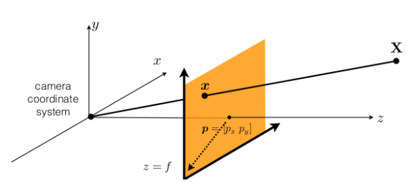
Four stages take a world point to a pixel: the extrinsics re-express it in the camera frame, perspective division flattens it onto the $z = 1$ plane, the lens bends it, and $K$ scales it into pixels.

Or compactly, $p = K \mathbin{@} d(\pi([R \mid t] \mathbin{@} X))$, where $\pi$ is the perspective division and $d(\cdot)$ the lens distortion. Note the matrix form above omits $d(\cdot)$ — distortion is nonlinear and cannot be folded into the product:

2. Inverse Projection (2D → 3D)

Running the chain backwards recovers a ray, not a point. Depth is destroyed by the perspective division, so every point along that ray produces the identical pixel:

Undoing $K$ is a matrix inverse, but undoing the lens is not — the distortion model has no closed-form inverse and is solved by fixed-point iteration. cv2.undistortPoints(pts, K, dist_coeffs) with P=None does both and hands back normalized coordinates.

3. Coordinate Systems

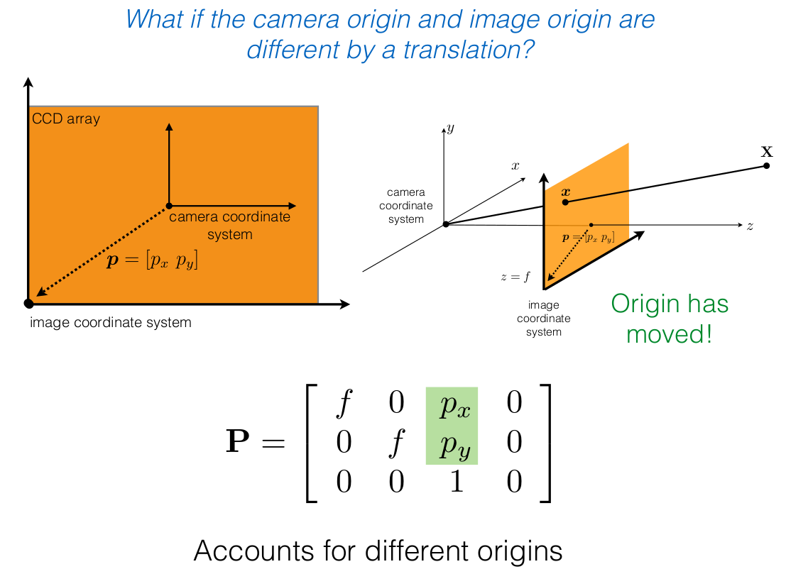
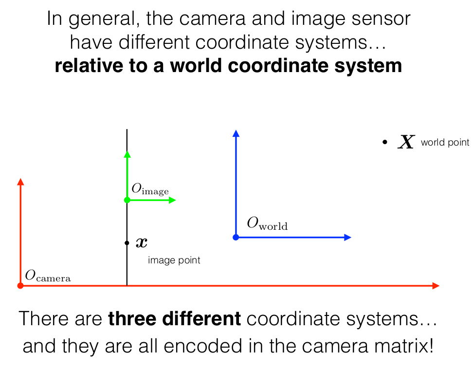
The camera projection model involves three coordinate systems:

1. World Coordinate Frame — the global 3D frame in which the scene lives.
2. Camera Coordinate Frame — centered at the optical center of the lens, with the z-axis pointing along the optical axis.
3. Image (Pixel) Coordinate Frame — the 2D plane onto which 3D points are projected, measured in pixels.

4. Hand-Eye Calibration

A camera bolted to a robot’s wrist has a nominal mounting transform, but tolerances and human error mean the real one is a few millimetres and a degree or two off. Hand-eye calibration recovers it.

The Setup

We have three transforms:

• $T_{Ref \to End}(i)$ — from forward kinematics on the joint encoders. Known.
• $T_{End \to Cam}$ — the camera mount. Rigid, but imprecisely known. This is $X$.
• $T_{Cam \to Board}(i)$ — from detecting checkerboard corners and running PnP. Known.

We need to find $T_{End \to Cam}$.

Bolt the base and the board down and the chain closes into a loop, so $T_{Ref \to Board}$ is a fixed quantity the arm cannot influence no matter how it moves:

Taking multiple samples we get

Both sides are the same constant, so the unknown mount is trapped between two measured quantities. Peel them off one side at a time.

Step 1 — left-multiply both sides by $T_{Ref \to End}(j)^{-1}$:

Step 2 — right-multiply both sides by $T_{Cam \to Board}(i)^{-1}$:

The unknown now stands alone on both sides, with a purely measured product to its left on one side and to its right on the other. Only now is it worth naming things:

Step 3 — substitute:

which is the classic $AX = XB$ problem: $A$ is the relative end-effector motion between the two poses, $B$ the relative camera motion, and $X$ the mount you want. A single pair leaves $X$ underdetermined, so capture $N \geq 15$ poses with plenty of rotation about different axes and non-coplanar viewpoints. The resulting system is overdetermined and solved as:

R_EndEffector_to_Camera, t_EndEffector_to_Camera = cv2.calibrateHandEye(
    R_robot_to_EndEffector_list,   # list of rotation matrices
    t_robot_to_EndEffector_list,   # list of translation vectors
    R_camera_to_checkerboard_list,
    t_camera_to_checkerboard_list,
    method=cv2.CALIB_HAND_EYE_TSAI  # or PARK, HORAUD, ANDREFF, DANIILIDIS
)

Refining with Reprojection Error (Optional)

Reprojection error measures how well the estimated transforms predict the observed image. For each checkerboard corner:

reprojection_error = || projected_2D - detected_2D ||

This polishes the closed-form solution, and the residual doubles as your validation metric.