• Introduction
• Part 1: The metric axis
  • The ambiguity nobody can escape
  • The fix: one canonical camera
  • Why it’s only half the story
• Part 2: The distortion axis
  • The pinhole plane runs out of room
  • What the degradation actually looks like
  • Option A: put every ray on a sphere (ERP)
    • The clever bit: fake a fisheye from perspective data
    • What ERP buys, and what it costs
  • Option B: don’t resample, predict the rays (SH ray fields)
    • Radial distance, not depth
    • What it costs
    • Side by side
• Part 3: Putting both fixes in one pipeline
  • Why this counts as a “composition”
  • What DAC actually says about it
  • The focal length of an image with no lens
• Part 4: Which one should you reach for?
  • An aside: “rays” does not mean “SH rays”
  • When to promote SH rays
• Takeaways
• References

Introduction

The camera models post ends with a pinhole, a matrix $K$, and a distortion function $d(\cdot)$ bolted onto the side because it refuses to fold into the matrix product:

\[p \;=\; K \mathbin{@} d(\pi([R \mid t] \mathbin{@} X)).\]

That $d(\cdot)$ is the awkward one. The classical recipe for dealing with it:

1. Fit a handful of radial and tangential coefficients to a checkerboard.
2. Invert them by fixed-point iteration — there’s no closed form.
3. Undistort the image, and carry on pretending you had a pinhole all along.

That works fine at 60°. It falls apart at 140°. It is meaningless at 200°.

Modern depth models don’t undistort at all. They change the representation so that distortion never becomes a problem in the first place — and in doing so they split what looks like one problem into two separate ones that people routinely conflate:

Axis	The problem	The fix
Metric scale	a wide lens and a narrow lens disagree about how many metres a pixel is worth	canonical-focal rescaling
Distortion	a flat image plane physically cannot hold a wide field of view	resample onto a sphere (ERP), or predict the rays directly (SH)

I’ll call these two things axes throughout — meaning two independent aspects of the problem that get fixed by separate mechanisms. Not directions on a graph; nothing here is plotted. The only thing the word is doing is insisting that these are two problems and not one.

And they really are independent: fixing either leaves the other exactly as it was. That’s what lets you fix them in separate places in the same pipeline, which is where almost every recent wide-FOV depth paper lands. The rest of this post takes them one at a time, then puts them back together.

---

Part 1: The metric axis

The ambiguity nobody can escape

Monocular depth is ill-posed for a reason that has nothing to do with neural networks:

• A small nearby object and a large faraway object project to exactly the same pixels.
• Add a second free variable — focal length — and it gets worse. A long lens looking at a far object and a short lens looking at a near object can be pixel-for-pixel identical.

If the image is the same, a network that only sees the image has no way to know which depth is correct. This is metric ambiguity, and it’s what makes “just predict metres” so fragile the moment you deploy on a camera whose focal length the model never saw.

The source is one line of the projection chain. For a 3D point $X$ at depth $Z$,

\[u \;=\; f\frac{X}{Z}.\]

Look at the fraction:

• $u$ depends only on the ratio $fX/Z$ — never on $f$ and $Z$ separately.
• Scale $f$ up and $Z$ up by the same factor, and $u$ doesn’t move at all.
• So the image is blind to any change that preserves $fX/Z$.

That’s why a network trained at one focal length systematically mis-reads depth at another. It’s a bias baked in by geometry, not by the data.

The fix: one canonical camera

Metric3D’s canonical-space trick is disarmingly simple. Pick one canonical focal length $f_c$ — a single virtual camera that everybody gets mapped into — and define a per-image rescale factor $\omega$:

\[\omega \;=\; \frac{f_c}{f}, \qquad Z_c \;=\; \omega Z, \qquad Z \;=\; \frac{1}{\omega}Z_c.\]

As a recipe:

• Train the network to predict the rescaled depth $Z_c = (f_c/f)\,Z$, never the raw $Z$.
• Every image lands in the same virtual camera before the loss is computed, whatever its native focal length — so the network only ever has to learn depth for one camera.
• Undo it at inference with $Z = (f/f_c)\,Z_c$, using the deployed camera’s real $f$.

That’s the entire transform: one scalar per image. It’s the reason a single model can serve many focal lengths.

The right-hand panel is worth a second look: plain image resizing is the same kind of operation. Scaling an image is geometrically indistinguishable from moving the object, so any resize in your data pipeline is silently a depth rescale too. That’s a good check on whether you’ve internalised the ambiguity — and an easy way to introduce a quiet bug if you haven’t.

Why it’s only half the story

Canonical-focal rescaling is a global similarity on a pinhole camera — it multiplies depth by one number for the whole image. So:

• ✅ It fixes scale. The systematic bias from a focal-length mismatch disappears.
• ❌ It cannot represent radial distortion. A single $\omega$ can’t make the periphery of a 140° lens behave, because the distortion out there isn’t a uniform rescale — it’s a per-pixel warp.

Canonical-focal owns exactly one axis. The other needs a different tool entirely.

Part 1 in one line. $u = fX/Z$ means the image only ever sees the ratio, so focal length and depth trade off invisibly. Rescaling everything to one canonical focal length collapses that trade-off into a single virtual camera — fixing scale, but not distortion.

---

Part 2: The distortion axis

The pinhole plane runs out of room

Here’s the problem in one sentence: a flat image plane cannot hold a wide field of view.

Go back to the pinhole relation for a ray at angle $\theta$ off the optical axis. It lands on the image plane at radius

\[r \;=\; f\tan\theta.\]

Watch what $\tan\theta$ does as the ray swings outward:

Ray angle $\theta$	$\tan\theta$	What happens on the plane
30°	0.58	comfortable
60°	1.73	already 3× further out than 30°
70°	2.75	badly stretched
89°	57.3	effectively off the sensor
90°	∞	no home at all

A pinhole has nowhere to put peripheral rays — and a 140° lens is all periphery ($\pm 70°$).

This is why a perspective-trained depth model degrades so hard on fisheye input. Two things go wrong at once:

• It was never shown the distorted periphery during training.
• The pinhole representation can’t even express it — so no amount of extra data fixes this on its own.

What the degradation actually looks like

That’s the argument. Here’s the measurement — DAC ran a perspective-trained metric depth model (Metric3D-v2) on the same scene presented five different ways:

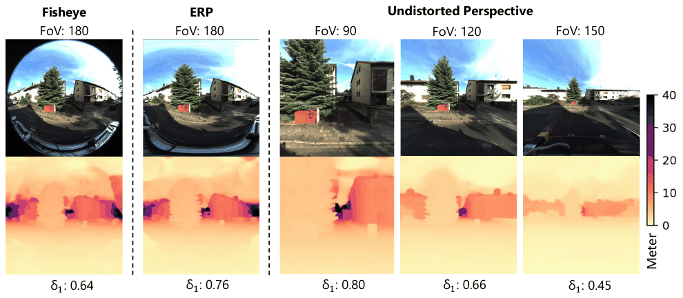
Read the $\delta_1$ row left to right — it’s the whole motivation for this post in five numbers:

Representation	FoV	$\delta_1$	What it tells you
Raw fisheye	180°	0.64	feed the distorted image straight in and the model struggles
ERP	180°	0.76	same 180° of content, just re-laid-out — and a big chunk of the loss comes back
Undistorted perspective	90°	0.80	the best score, but you threw away most of the field of view to get it
Undistorted perspective	120°	0.66	pushing the undistortion wider starts to hurt
Undistorted perspective	150°	0.45	now it’s far worse than just feeding the raw fisheye

Three things fall out of that table:

• The “just undistort it” escape hatch works — but only by throwing away FOV. 0.80 at 90° is the best number on the board, and it’s the one where you’ve discarded the wide-angle coverage you bought the lens for.
• Undistorting wide is actively counterproductive. By 150° it scores 0.45, well below the 0.64 you’d get by not undistorting at all. $r = f\tan\theta$ stretches the periphery so violently that the resampled image is worse input than the original.
• ERP gets most of it back for free. At the full 180°, ERP scores 0.76 — beating undistorted perspective at 120° and 150°, using the same model with no retraining. That single comparison is the case for the whole distortion axis.

Note what’s being measured: this is the baseline degrading, not DAC’s own result. The model is perspective-trained throughout; only the input representation changes. Which is precisely why it isolates the representation effect from the training-data effect.

Option A: put every ray on a sphere (ERP)

The fix is to stop insisting on a flat plane:

1. Map every pixel to a direction on the unit sphere — a latitude $\phi$ and a longitude $\lambda$.
2. Unroll that sphere into an equirectangular projection (ERP): a plain 2D grid of $(\lambda, \phi)$.

There’s no $\tan\theta$ anywhere in that, so nothing blows up. Every ray, however far off-axis, gets an evenly-spaced cell, and a 140° cone maps to a bounded band of latitudes with room to spare.

Going the other way — from an ERP cell back to the pixel it came from — uses the gnomonic projection about a tangent centre $(\lambda_c, \phi_c)$:

\[x_t \;=\; \frac{\cos\phi\,\sin(\lambda-\lambda_c)}{\cos c}, \qquad \cos c \;=\; \sin\phi_c\sin\phi + \cos\phi_c\cos\phi\cos(\lambda-\lambda_c).\]

Don’t memorise it. Only two properties matter:

• It’s closed-form — no iteration, unlike inverting a classical distortion model.
• For each cell in the ERP patch, it names the exact floating-point location in the source image to interpolate from. In other words, it’s just a grid-sample.

ERP is a resampling front-end, not a new network.

The clever bit: fake a fisheye from perspective data

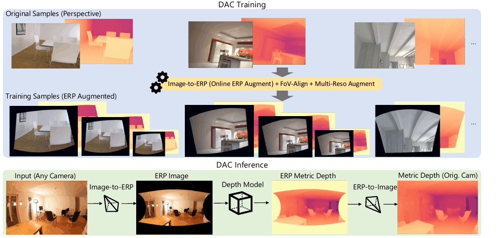
Depth Any Camera (DAC) turns this into a training strategy. Because the gnomonic map is parameterised by the tangent centre $(\lambda_c, \phi_c)$, you can tilt it:

• Set $\lambda_c = 0$ and a perspective patch lands in the low-distortion band, near the equator.
• Set $\lambda_c \neq 0$ and the same patch lands in the high-distortion band — exactly the region a wide fisheye would observe.

So you can take ordinary perspective training images and, on the fly, project them into fisheye-like distortion without owning a fisheye camera.

The whole DAC recipe is three ingredients:

• Pitch-aware Image-to-ERP conversion — the tilt trick above.
• FoV-Align — normalise every camera’s data to one predefined ERP patch size.
• Multi-resolution augmentation — so the model survives the train/test resolution gap.

Trained exclusively on perspective data, it generalises zero-shot to fisheye and 360°, improving $\delta_1$ accuracy by up to 50% over Metric3D-v2 / UniDepth on large-FOV benchmarks.

What ERP buys, and what it costs

• ✅ Cheap. A grid-sample sitting in front of whatever depth backbone you already have.
• ✅ Non-invasive. The entire loss stack — scale-and-shift-invariant loss, gradient matching, temporal consistency — is untouched, because from the network’s point of view it’s still just predicting depth on an image.
• ✅ Free training data. The tilt trick manufactures fisheye supervision out of perspective datasets you already have.
• ❌ Needs the camera model at test time to build the patch. For a genuinely uncalibrated lens that’s a real problem — and it’s the opening for the alternative.

Option B: don’t resample, predict the rays (SH ray fields)

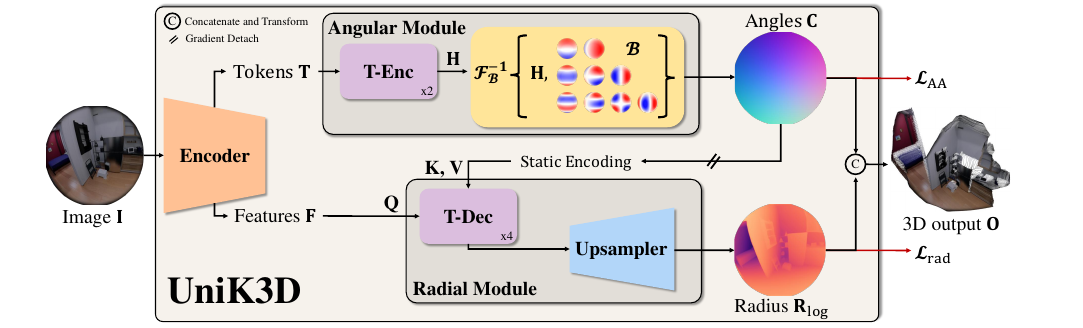
UniK3D asks the obvious follow-up: why resample at all? Why not let the network predict the camera’s rays directly and skip the intermediate image entirely?

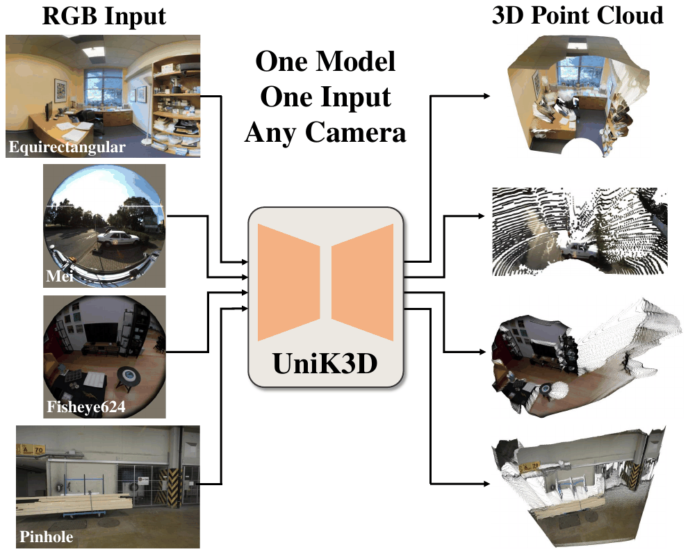
Every camera — pinhole, fisheye, 360°, anything — is fully described by its pencil of rays: the map from each pixel to the 3D direction it looks along.

• A pinhole’s rays fan out mildly.
• A fisheye’s bend sharply at the edges.
• If you know the ray field, you know the camera. No intrinsics required.

UniK3D predicts that ray field as a learned superposition of spherical harmonics. An angular module emits a small set of coefficients $\mathbf{H}$, and ray directions come back via an inverse spherical-harmonic transform:

\[\mathbf{C} \;=\; \mathcal{F}_{\mathcal B}^{-1}\{\mathbf H\} \;=\; \sum_{l=0}^{L}\sum_{m=-l}^{l} \mathbf H_{lm}\,\mathcal B_{lm}(\theta, \phi).\]

Two things worth pausing on:

• The basis functions $\mathcal B_{lm}$ are fixed and known — the low-order “lobes” you see in the animation. Only the coefficients $\mathbf H_{lm}$ are predicted.
• A basis up to degree 3 with no constant term needs just 15 coefficients to describe the ray field of essentially any camera. That’s a remarkably compact way to say “here’s how this lens bends light.”

Radial distance, not depth

There’s a second, subtler design choice hiding in that figure: UniK3D predicts radial distance along each ray — true Euclidean distance from the camera centre — rather than perpendicular depth $Z$. Why?

• Past a 90° field of view, perpendicular depth becomes ill-conditioned. The $Z$ of a ray pointing almost sideways is a strange quantity, and at exactly 90° it’s degenerate.
• Radial distance stays well-behaved at any angle. It’s just “how far along this ray.”

That one choice is what keeps the representation well-posed past 180°, where both ERP and pinhole start to break down.

Credit where due, though: this move isn’t the SH camp’s private insight. DAC makes exactly the same switch on the ERP side — its depth is “represented as Euclidean Distance from the camera center rather than Z-buffer format, as the latter is incompatible with spherical projections.” Any spherical representation forces it. What stays genuinely UniK3D’s is the part that comes next: the rays themselves are predicted, not given.

What it costs

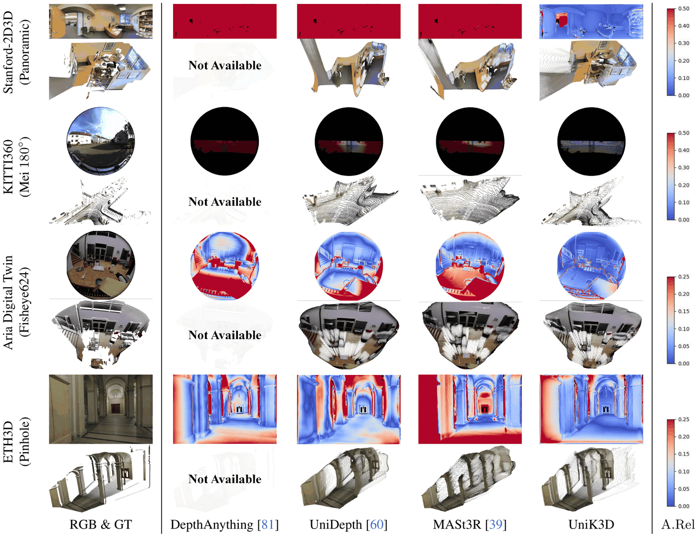
Two clear wins over ERP:

• ✅ Calibration-free at test time. The network predicts the rays, so it needs no intrinsics, no rectification, no known camera model. Hand it an image and it figures out the lens.
• ✅ Well-posed beyond 180°. Radial distance plus spherical rays don’t blow up at extreme FOV. For genuinely omnidirectional cameras this is decisive.

Neither is free:

• ❌ Bespoke architecture. A dedicated angular module, a radial module conditioned on it, a spherical-harmonic output space, and a matching asymmetric angular loss.
• ❌ Different output geometry. It emits radial 3D, not the affine-invariant depth map most video-depth loss stacks are built around.
• ❌ Not a drop-in. You can’t bolt it onto a depth foundation model as “just a LoRA” — it replaces the head and the loss geometry.

When those advantages do bind, though, the gap is not subtle:

Side by side

	ERP / gnomonic	SH ray field
What it is	resampling front-end	learned output representation
Touches the backbone?	no — grid-sample in front	yes — replaces head and losses
Needs intrinsics at test time?	yes	no
Valid past 180°?	no	yes
Output	Euclidean distance on the ERP grid — metric after canonical rescale	radial distance + rays
Training data	manufacture fisheye from perspective	needs its own regime
Representative work	Depth Any Camera	UniK3D, CAM3R

Part 2 in one line. ERP is a cheap front-end that preserves your whole pipeline; SH rays are a more powerful but more invasive rebuild.

---

Part 3: Putting both fixes in one pipeline

So far the two fixes have been described separately. The natural worry is that they’ll fight each other once you use both. They don’t — and it’s worth being precise about why, because “they’re orthogonal” is the sort of phrase that sounds like an explanation without actually being one.

Here is the whole thing as a single pipeline, with the two fixes marked:

flowchart LR
    A["<img src='/images/blog/computer-vision/beyond-the-pinhole-camera/glyph-fisheye.svg' width='90'/><b>fisheye frame</b>"]
    B["<img src='/images/blog/computer-vision/beyond-the-pinhole-camera/glyph-erp.svg' width='90'/><b>ERP patch</b>"]
    C["<img src='/images/blog/computer-vision/beyond-the-pinhole-camera/glyph-depth.svg' width='90'/><b>canonical depth</b><br/><i>canonical-camera metres</i>"]
    D["<b>metric depth</b><br/><i>metres</i>"]

    A -- "<span style='color:#7ddba0;font-weight:700'>FIX 1 · distortion</span><br/>ERP grid-sample" --> B
    B -- "depth network" --> C
    C -- "<span style='color:#5fa87c;font-weight:700'>FIX 2 · scale</span><br/>× f<sub>virt</sub> / f<sub>cano</sub>" --> D

    classDef stage fill:#1a1d27,stroke:#2a2d3a,color:#e0e0e6;
    class A,B,C,D stage;

Why this counts as a “composition”

Composition in the ordinary function-composition sense: two operations applied one after another, where neither disturbs what the other did. That property isn’t automatic — it has to be earned, and here it’s earned by the two fixes rewriting different variables.

	Fix 1 — ERP grid-sample	Fix 2 — canonical rescale
What it rewrites	pixel coordinates — where each ray lands	depth values — what the numbers mean
What it leaves alone	the depth numbers (still arbitrary units)	the ray geometry (not one pixel moves)
Kind of operation	a per-pixel resampling	a single scalar for the whole image

That’s why the diagram reads left to right with no crossing arrows. ERP re-lays-out the image and does nothing to put depth into metres; the rescale multiplies the depth map by one number and does not move a single ray. Apply both and you end up with both fixed — and since neither reads the other’s variable, the order you apply them in genuinely doesn’t matter.

That is all “orthogonal” was ever claiming. Not “unrelated”, but disjoint in what they modify.

What DAC actually says about it

Worth being straight about the sourcing here: DAC has no single figure for this composition — the diagram above is mine. The paper splits the two halves across two figures that never meet:

• Figure 3 shows the depth scaling, with no ERP anywhere in it.
• Figure 4 shows the ERP pipeline, and its inference row — input → Image-to-ERP → depth model → ERP-to-Image — doesn’t draw the rescale step at all.

The composition itself appears once, as a line of prose in the preliminaries: the canonical depth-scaling operations “are central to the Metric3D pipeline and are integrated into our ERP-based approach.” So it is genuinely how DAC is built — just never drawn in one place.

The focal length of an image with no lens

There’s one detail the compact story skates over, and it’s the natural objection to the whole composition: fix 2 multiplies by a ratio of focal lengths — but which focal length? The ERP patch was built by a grid-sample. Whatever $f$ the original lens had is gone; ERP cells are indexed by angle, not by any focal length.

DAC’s answer is to read a virtual focal length off the ERP grid itself:

\[\frac{1}{f_{virt}} \;=\; \tan\!\left(\frac{\pi}{H_{erp}}\right).\]

That’s just the pinhole relation $r = f\tan\theta$ run backwards for a single cell: an ERP image of height $H_{erp}$ spans 180° of latitude, so one row subtends $\pi/H_{erp}$ radians, and $f_{virt}$ is the focal length of the pinhole camera for which that angle lands exactly one pixel from centre. Angular resolution has taken over the role the lens used to play.

The rest is Part 1 verbatim, with $f_{virt}$ standing in for $f$: training depth is scaled by $f_{cano}/f_{virt}$ (DAC uses $f_{cano} = 519$ indoor and $721$ outdoor, with $H_{erp} = 1400$), and inference multiplies predictions by $f_{virt}/f_{cano}$ to get metres back. Fisheye inputs are converted to ERP first and scaled through $f_{virt}$ too — the paper notes that trying to align $f_{cano}$ with a fisheye’s post-distortion focal length directly “introduces significant errors.”

Written compactly:

\[\underbrace{\text{image} \xrightarrow{\;\text{gnomonic grid-sample}\;} \text{ERP patch}}_{\textbf{fix 1: distortion}} \;\longrightarrow\; \text{depth net} \;\longrightarrow\; \underbrace{\hat Z \xrightarrow{\;\times\, f_{virt}/f_{cano}\;} Z}_{\textbf{fix 2: scale}}\]

What that modularity buys you in practice:

1. Solve the hard axis first. Distortion (ERP) is the load-bearing part — it’s what lets a narrow-FOV-trained model transfer to a wide lens at all.
2. Add the metric axis only if you need it. In DAC itself the metric axis is integral, not bolted on: the network trains against metric ground truth in canonical space, and the rescale is what connects that space back to real metres. But the pattern doesn’t force the choice on you — if your target is affine-invariant, with absolute scale recovered downstream from triangulation, LiDAR, or a known baseline, you can train a relative model on ERP patches and fix 2 never exists. That’s a departure from DAC, not a description of it.
3. Neither disturbs your losses. Both are pre/post transforms around the network, not changes to it.

Part 3 in one line. One fix rewrites pixel coordinates, the other rewrites depth values — different variables, so neither can undo the other. That’s what lets them sit at opposite ends of one pipeline and be staged independently.

---

Part 4: Which one should you reach for?

flowchart TD
    Q1["<b>Field of view &gt; 180°?</b><br/><i>omnidirectional / panoramic</i>"]
    Q2["<b>Can the lens be calibrated?</b><br/><i>even once, offline</i>"]
    Q3["<b>Monocular depth, or<br/>feed-forward reconstruction?</b>"]
    ERP["<b>ERP front-end</b><br/>Depth Any Camera<br/><i>grid-sample, no retrain</i>"]
    PM["<b>pointmap / ray-map head</b><br/>VGGT · Pi3 · MapAnything · DA3<br/><i>rays, but not SH</i>"]
    SH["<b>SH ray field</b><br/>UniK3D · CAM3R<br/><i>calibration-free,<br/>well-posed past 180°</i>"]

    Q1 -- "no" --> Q2
    Q1 -- "yes" --> SH
    Q2 -- "yes, once" --> Q3
    Q2 -- "never" --> SH
    Q3 -- "depth" --> ERP
    Q3 -- "reconstruction" --> PM

    classDef q fill:#1a1d27,stroke:#6c9eff,color:#e0e0e6;
    classDef rec fill:#17301f,stroke:#2e8b57,color:#e0e0e6;
    classDef sh fill:#2a2340,stroke:#8b5cf6,color:#e0e0e6;
    class Q1,Q2,Q3 q;
    class ERP,PM rec;
    class SH sh;

Take the concrete case that motivates most of this work: you train on ~80–90° perspective data and deploy on a ~140° fisheye. Do you need the spherical-harmonic machinery, or is ERP enough?

Short answer: ERP is enough, and it’s probably the right call. Four reasons, heaviest first.

1. 140° is comfortably below 180°. The single biggest reason to prefer SH rays is that radial distance plus spherical output stay well-posed past 180°. If you never go past it, ERP/gnomonic is fully well-posed across the entire cone — the pole-region distortion and sample-waste that hurt ERP live beyond where your camera ever looks. SH’s headline advantage simply isn’t in play.
2. ERP is non-invasive; SH rays are a rebuild. ERP is a grid-sample in front of the backbone, so architecture and losses stay untouched. SH replaces the output head and the loss geometry — a poor fit for a low-data adaptation regime (LoRA and friends).
3. The metric axis composes for free. ERP stacks cleanly with canonical-focal rescaling, so a near-metric prior can be added later without touching the front-end. That modularity is what a staged, risk-managed plan wants.
4. Calibration is a one-time cost. ERP’s one real weakness is needing the camera model. But you can calibrate the lens once (Kannala–Brandt, or the vendor model) and plug it into the ERP front-end with no retraining — the design was built for an unseen wide camera, and calibration just fills in the last parameter.

An aside: “rays” does not mean “SH rays”

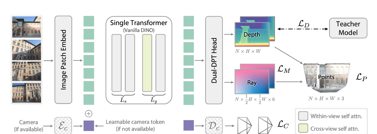
Worth flagging, because it’s an easy conflation. If you’re doing feed-forward reconstruction rather than monocular depth, the reasoning goes: a pointmap is already ray × distance, so the ray head belongs inside the network. The premise is true; the conclusion doesn’t follow. Look at what the field-leading feed-forward reconstructors actually use:

Model	Camera / geometry representation	SH ray field?
VGGT	parametric intrinsics/extrinsics + pointmaps	❌
Pi3	pointmaps + poses (reference-free)	❌
MapAnything	dense ray map + depth + pose + scale	❌
Depth Anything 3	depth-ray (dense depth + ray map) — beats pointmaps	❌
Wid3R	camera-model token conditioning	❌
UniK3D	SH ray field + radial distance	✅
CAM3R	SH rays + radial distance	✅

Reading that table:

• MapAnything and DA3 do factor geometry through rays — and still avoid spherical harmonics. DA3 even reports that its ray-map target beats pointmaps.
• “Inside the network” is satisfied by a plain dense ray map, or by raw pointmaps. Neither one is SH.
• SH is a niche whose only two payoffs — calibration-free, well-posed past 180° — don’t bind on a calibratable sub-180° lens.

When to promote SH rays

The reserve isn’t decorative. It’s gated on two triggers:

Trigger	Why SH rays win there
The lens can never be calibrated	calibration-free ray prediction earns its complexity
FOV creeps past ~180°	ERP degrades; radial + spherical stays well-posed

Note what’s not on that list: “we’re doing reconstruction instead of depth.” That’s an architecture question, not a camera-model question.

There’s also a cheap hedge that commits you to neither: Calibration Tokens.

• Roughly 8 learned tokens per layer, under 1 MB, sub-millisecond.
• Self-supervised, and requires no fisheye training images.
• Hands a perspective-domain model fisheye robustness while keeping the output pinhole.
• Backward-compatible: omit the tokens and you get the original perspective model back, unchanged — so it costs you nothing on in-domain data.

Useful if you suspect an in-domain perspective model might still win.

---

Takeaways

• Two orthogonal problems. $u = fX/Z$ means focal length and depth trade off invisibly (metric axis); $r = f\tan\theta$ means a flat plane can’t hold a wide FOV (distortion axis). Don’t conflate them.
• Metric axis: canonical-focal rescaling. $Z_c = (f_c/f)Z$ collapses every camera into one virtual camera. One scalar. Fixes scale, cannot touch distortion.
• Distortion axis, option A: ERP. A closed-form gnomonic grid-sample front-end. Leaves the network and losses intact, and tilting the tangent centre lets you manufacture fisheye distortion from perspective data. Needs the camera model at test time.
• Distortion axis, option B: SH ray fields. Predict the pencil of rays as 15 coefficients and output radial distance. Calibration-free and well-posed past 180°, but a bespoke architecture that replaces the head and the losses.
• They compose. ERP in front, canonical rescale behind, one network in the middle — which is exactly what DAC does, with a virtual focal length read off the ERP grid’s angular resolution standing in for the lens’s $f$.
• Default: below 180° and calibratable, take ERP (or a pointmap/ray-map head if you’re doing feed-forward reconstruction). Keep SH in reserve for the two triggers that actually justify it.

For the underlying projection algebra — forward and inverse projection, the classical distortion model, coordinate frames, and hand-eye calibration — see the Camera Models appendix.

---

References

• Guo et al., Depth Any Camera: Zero-Shot Metric Depth Estimation from Any Camera, CVPR 2025 — arXiv:2501.02464
• Piccinelli et al., UniK3D: Universal Camera Monocular 3D Estimation, CVPR 2025 — arXiv:2503.16591
• Yin et al., Metric3D: Towards Zero-shot Metric 3D Prediction from A Single Image, ICCV 2023 — arXiv:2307.10984
• Wang et al., VGGT: Visual Geometry Grounded Transformer, CVPR 2025 — arXiv:2503.11651
• Calibration Tokens: Adapting Foundation Depth Models for Fisheye Cameras — arXiv:2508.04928

All paper figures above are reproduced from the linked arXiv preprints and are credited in their captions.