• Introduction
• Part 1 : Volume Rendering
  • Understanding Absorption and Trasmittance
    • Absorption Emission Model
    • Absorption-only Model
    • Why The Importance on Transmittance
    • Emission-Absorption Transmittance
    • Ray Marching
    • Practice Transmittance Calculations
    • Implementing Ray Marching
      • 1. Discretize the space into small volumes (just define the sampling points)
      • 2. Get the density and color of each small volume (This step is Done by the NERF MLP.)
      • 3. Aggregate the density and color of each small volume to get the final color at the origin of each ray
      • NOTE:
• Part 2 : NERF Pipeline
  • Overview:
  • NeRF Training Loop (Simple)

Introduction

NERF gave us a whole new way of approaching general computer vision tasks like Novel View Synthesis (NVS), 3D Reconstruction, etc. in a more physics informed way.

The NeRF is basically an MLP that learns the 3D density and 5D light field of a given scene from image observations and corresponding perspective transforms.

Q. What’s 5D Light Field?

Ans. Choosing any ray (i.e. choosing any starting origin and direction) in the scene,
     we should be able to find the total radiance coming from that ray.

Q. What is Radiance?

Ans. Measure of Radiant Energy (joules) per unit time, per unit area, per unit solid angle
     AKA: The amount of irradiance per unit solid angle

Since the formulation of rendering is crucial to understanding NERFs we’ll do that first.

Part 1 : Volume Rendering

Understanding Absorption and Trasmittance

Absorption Emission Model

Let’s consider an infinitesimal (small) volume through which we have a light ray travelling. Now, this volume can do two things:

• Absorb some intensity of incoming light
• Emit some light of it’s own

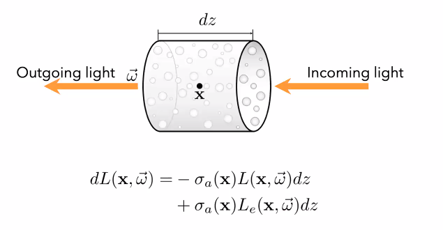
For both cases, we see the factor σ this is the absorption coefficient of the volume. Furthermore, we see that both incoming light and light produced in this volume will be affected by this σ

Absorption-only Model

Modelling only absoroption through a non-homogenous volume, we derive the relationship between incoming radiation and outgoing radiation as follows:

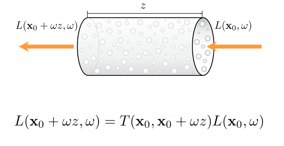
Note in above figure, x0 is where the light ray enters the volume. We assume the volume is perfectly oriented in the ray’s direction ω. Then ωz would be the length of the volume along the ω unit vector. That’s why the final radiance output is L(x0 + ωz, ω)

As you can observe, we have a new term here called Transmittance. The intuitive meaning of transmittance is the proportion of incoming light that eventually leaves the volume (gets transmitted).

Think of it like absorption is a coefficient (say 0.2) meaning that 20% of all incoming light is absorbed. For transmittance (say 0.8) the intuition would be that 80% of all light is let through the medium.

Why The Importance on Transmittance

Trasmittance has some nice properties which simple absorption would not have. Specifically:

• Monotonic Function
• Multiplicativity

In the below picture, we see that even though σ might vary in the volume, the transmittance is always a monotonic function:

Now, previously we saw Transmittance for a non-homogenous medium. It can be easily adapted to a homogenous medium as well as shown below:

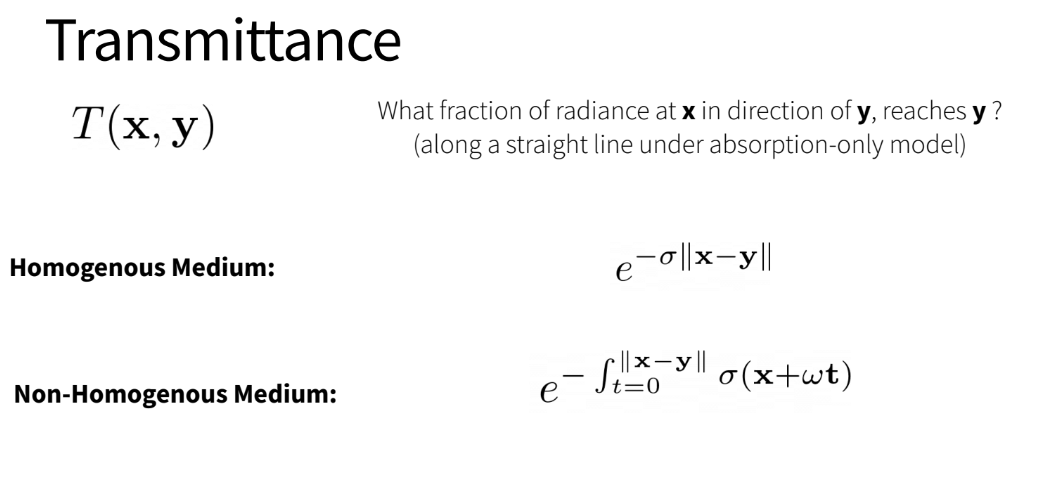
Now, above we see that it’s basically an exponential. The multiplicativity property of transmittance is due to the this multiplicativity of exponentials

Using our transmittance terminology above, we finnaly get for absorption only transmittance:

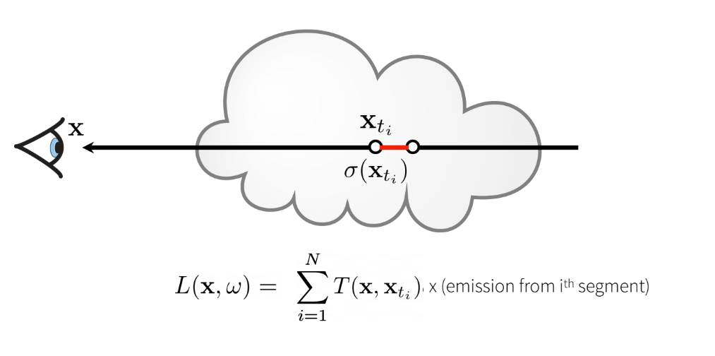
Emission-Absorption Transmittance

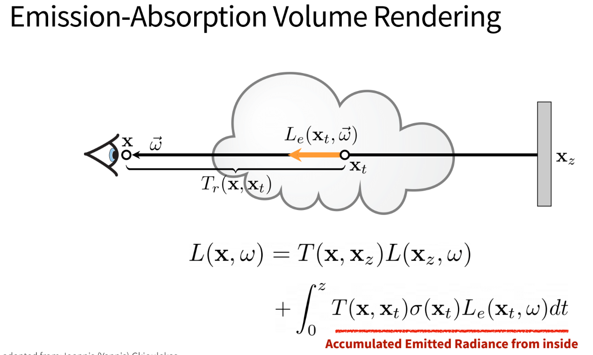
As a recap of what was done above, let’s see the basic absorption model

In the above picture note the following:

• The transmittance in vacuum is 1
• Only the cloud has some transmittance value less than 1
• Therefore T(x,x_z) = T_cloud in the above scenario

Now, lets make some assumptions to go from absorption only model to absorption-emission model:

• Let’s divide the cloud into small sections (small volumes)
• Let each volume not only absorb (have transmittance < 1) but also be able to emit light
• The final radiation at the eye will be a combination of emission and absorption

The context above is baked into the picture below:

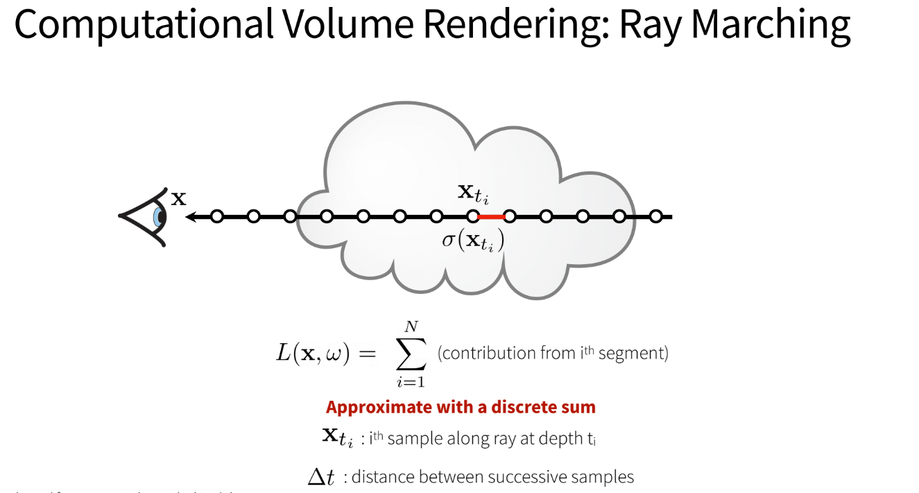
Ray Marching

Now, the issue with the emission-absorption model is that the integral cannot be solved numerically without some simplifications. We will make the following simplifications:

• Discretize the space into small volumes
• Let each small volume have it’s own σ
• Our final radiation at the eye/camera will be the summation of each of these small volumes

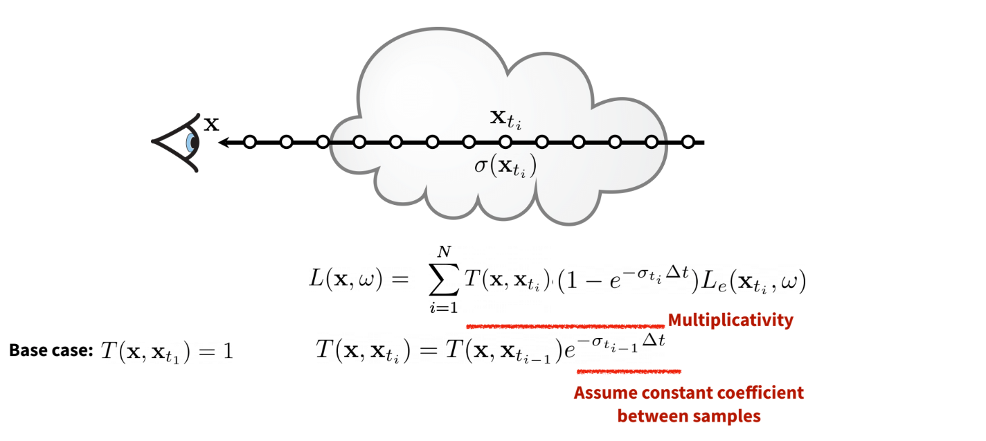
Finally, we see that computing Transmittance is recursive, where the i+1’th segment’s transmittance (T_i+1) = T(i) * T(small volume of i+1)

Practice Transmittance Calculations

Implementing Ray Marching

This will be done in two steps:

1. Discretize the space into small volumes (just define the sampling points)

import torch
from ray_utils import RayBundle
from pytorch3d.renderer.cameras import CamerasBase


# Sampler which implements stratified (uniform) point sampling along rays
class StratifiedRaysampler(torch.nn.Module):
    def __init__(
        self,
        cfg
    ):
        super().__init__()

        self.n_pts_per_ray = cfg.n_pts_per_ray
        self.min_depth = cfg.min_depth
        self.max_depth = cfg.max_depth

    def forward(
        self,
        ray_bundle,
    ):
        # Compute z values for self.n_pts_per_ray points uniformly sampled between [near, far]
        z_vals = torch.linspace(self.min_depth, self.max_depth, self.n_pts_per_ray, device=ray_bundle.origins.device)

        # Sample points from z values
        """
        NOTE: if image_plane_points.shape = torch.Size([65536, 3]),
              then rays_origin.shape = torch.Size([65536, 3])
              and sample_lenths.shape = torch.Size([65536, 1, 3])
        """

        origins_expanded = ray_bundle.origins.unsqueeze(1)  # Shape: (N, 1, 3)
        origins_expanded = origins_expanded.expand(-1, self.n_pts_per_ray, -1)  # Shape: (N, D, 3)
        directions_expanded = ray_bundle.directions.unsqueeze(1)  # Shape: (N, 1, 3)
        directions_expanded = directions_expanded.expand(-1, self.n_pts_per_ray, -1)  # Shape: (N, D, 3)
        z_vals_expanded = z_vals.expand(ray_bundle.origins.shape[0], -1).unsqueeze(-1)  # Shape: (1, D, 1)

        new_sample_points = origins_expanded + z_vals_expanded * directions_expanded

        # Return
        return ray_bundle._replace(
            sample_points=new_sample_points,
            sample_lengths=z_vals_expanded * torch.ones_like(new_sample_points[..., :1]), # shape = (N, D, 1)
        )

2. Get the density and color of each small volume (This step is Done by the NERF MLP.)

3. Aggregate the density and color of each small volume to get the final color at the origin of each ray

NOTE:

During training, density is not explicitly trained for. Instead, we check what the final color of a ray should be and compare with what the NERF MLP is telling us. This comparison gives us our loss which will update ray marching.

Because we don’t optimize for density directly, that’s why the NeRF Depth output is bad. That’s what prompted people to move to Neural SDFs so that geometry would be better optimized.

Part 2 : NERF Pipeline

Overview:

• Define a set of rays (origin, direction):

  return RayBundle
  (
    rays_origin,
    rays_d,
    sample_lengths=torch.zeros_like(rays_origin).unsqueeze(1),
    sample_points=torch.zeros_like(rays_origin).unsqueeze(1),
  )
  

• Give rays (origin, direction) to StratifiedRaysampler to get the sample points along the rays
  • i.e. Do the discretization step of Ray Marching

    # Sample points along the ray
    cur_ray_bundle = StratifiedSampler(cur_ray_bundle)
    

• Pass the sample points to the NERF MLP to get the density and color of each sample point
  • Note: These sample points are anywhere along the rays (think of it like random camera positions and randomly close to the object) and we want to predict the density and color

    predictions = NeRF_MLP(cur_ray_bundle)
    

The next two steps are a bit involved

• Aggregate the density and color of each sample point to get the final color at the origin of each ray. (the final color of all rays forms the IMAGE!)
• Compare the final colors (Image) with the GT image to get the loss

Check out the forward function in the Volume Renderer class below reference:

Reference

predicted_density_for_all_samples_for_all_rays_in_chunk = NERF_MLP_output['density'] # shape = (self._chunk_size*n_pts, 1) : The density value of that discrete volume
predicted_colors_for_all_samples_for_all_rays_in_chunk = NERF_MLP_output['feature'] # shape = (self._chunk_size*n_pts, 3) : Emittance for each discrete volume for RGB channels

# Compute length of each ray segment
# NOTE: cur_ray_bundle.sample_lengths.shape = (self._chunk_size, n_pts, n_pts)
depth_values = cur_ray_bundle.sample_lengths[..., 0] # depth_values.shape = (self._chunk_size, n_pts)
# deltas are the distance between each sample
deltas = torch.cat(
    (
        depth_values[..., 1:] - depth_values[..., :-1],
        1e10 * torch.ones_like(depth_values[..., :1]),
    ),
    dim=-1,
)[..., None]

# Compute aggregation weights (weights = overall transmittance for all rays in the chunk)
weights = self._compute_weights(
    deltas.view(-1, n_pts, 1), # shape = (self._chunk_size, n_pts, 1)
    predicted_density_for_all_samples_for_all_rays_in_chunk.view(-1, n_pts, 1) # shape = (self._chunk_size, n_pts, 1)
)

# TODO (1.5): Render (color) features using weights
# weights.shape = (self._chunk_size, n_pts, 1)
# color.shape = (self._chunk_size*n_pts, 3)
color_of_all_rays = self._aggregate(weights, predicted_colors_for_all_samples_for_all_rays_in_chunk.view(-1, n_pts, 3)) # feature = RGB color

# TODO (1.5): Render depth map
# depth_values.shape = (self._chunk_size, n_pts)
depth_of_all_rays = self._aggregate(weights, depth_values.view(-1, n_pts, 1))

# Return
cur_out = {
    'feature': color_of_all_rays,
    'depth': depth_of_all_rays,
}
# shape = (N, 3) for feature and (N, 1) for depth

The function compute_weights will find the overall transmittance for each ray and compute_aggregate will use this transmittance to find either color or depth for each ray

def _compute_weights(
        self,
        deltas,
        rays_density: torch.Tensor,
        eps: float = 1e-10):
        """

        Args:
            deltas : distance between each sample (self._chunk_size, n_pts, 1)
            rays_density (torch.Tensor): (self._chunk_size, n_pts, 1) predicting density values of each sample (from NERF MLP)
            eps (float, optional): Defaults to 1e-10.

        Returns:
            _type_: _description_
        """
        # TODO (1.5): Compute transmittance using the equation described in the README
        num_rays, num_sample_points, _ = deltas.shape
        transmittances = []
        transmittances.append(torch.ones((num_rays, 1)).to(deltas.device)) # first transmittance is 1

        #! Find the transmittance for each discrete volume = T(x, x_i)
        for i in range(1, num_sample_points):
            # recursive formula for transmittance
            transmittances.append(transmittances[i-1] * torch.exp(-rays_density[:, i-1] * deltas[:, i-1] + eps))

        #! Find = T(x, x_t) * (1 - e^{−σ(x) * δx})
        transmittances_stacked = torch.stack(transmittances, dim=1)
        # the below line implements the T(x, x_t) * (1 - e^{−σ(x) * δx}) part of the equation => we'll call this 'weights'
        return transmittances_stacked * (1 - torch.exp(-rays_density*deltas+eps)) # -> weights

    def _aggregate(
        self,
        weights: torch.Tensor,
        rays_feature: torch.Tensor):
        """

        Args:
            weights (torch.Tensor): (self._chunk_size, n_pts, 1) (Overall Transmittance for each ray)
            rays_feature (torch.Tensor): (self._chunk_size*n_pts, 3) feature = color/depth

        Returns:
            feature : Final Attribute (color or depth) for each ray
        """
        # TODO (1.5): Aggregate (weighted sum of) features using weights
        feature = torch.sum((weights*rays_feature), dim=1)
        return feature

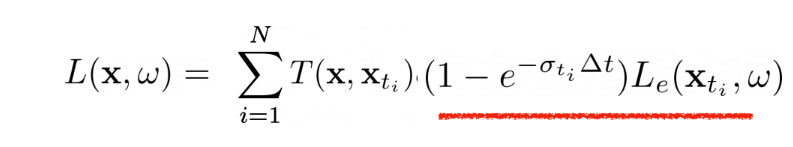
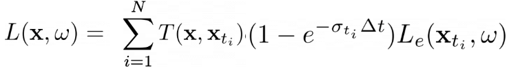
Basically, compute_weights finds the T(x, x_t) * (1 - e^{−σ(x) * δx}) part of the equation below:

And _aggreate finds the L(x,ω) which can be color or depth for each ray

NeRF Training Loop (Simple)

for iteration, batch in t_range:
            image, camera, camera_idx = batch[0].values()
            image = image.cuda().unsqueeze(0)
            camera = camera.cuda()

            # Sample rays
            xy_grid = get_random_pixels_from_image(
                cfg.training.batch_size, cfg.data.image_size, camera
            )
            ray_bundle = get_rays_from_pixels(
                xy_grid, cfg.data.image_size, camera
            )
            rgb_gt = sample_images_at_xy(image, xy_grid)

            # Run model forward
            out = model(ray_bundle)

            # TODO (Q3.1): Calculate loss
            loss = criterion(out['feature'], rgb_gt)

            # Take the training step.
            optimizer.zero_grad()
            loss.backward()
            optimizer.step()