Neural Nets are the ‘Policy’

Neural net as policy

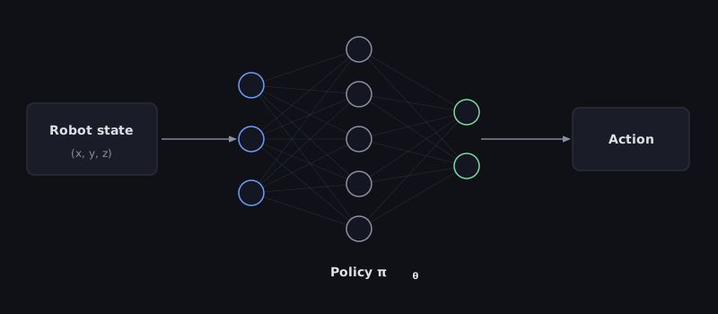
In the case of imitation learning or behaviour cloning this can be thought of as: given expert demonstrations, can we train a neural network (a policy) to mimic those actions? This turns out to be surprisingly nuanced. The way we design the model’s outputs and loss function has a huge impact on how “expressive” the learned policy can be.

This post walks through the progression from naive approaches to more expressive generative policies.

Discrete Actions: The Simple Case

Consider training a network to play Pacman.

Pacman policy

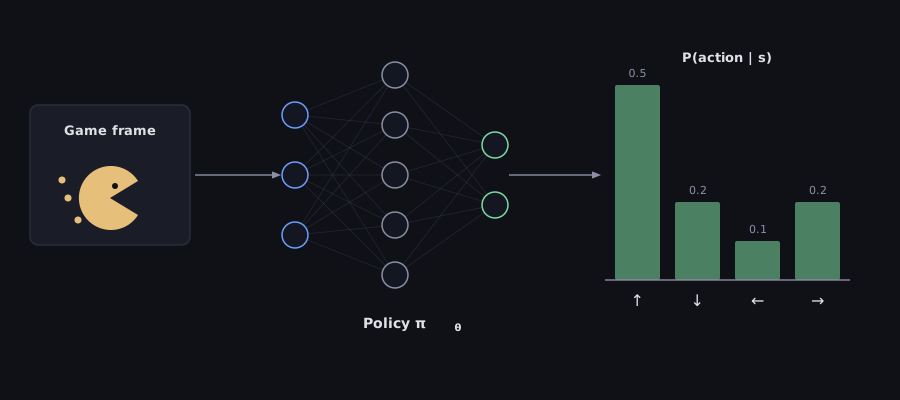
This is just a classification problem. The model outputs 4 logits (one per action), and we train with cross-entropy loss. Simple, clean, and maximally expressive i.e. the softmax output can represent any distribution over those 4 buttons.

But what happens when actions are continuous…?

Continuous Actions: Where Things Get Interesting

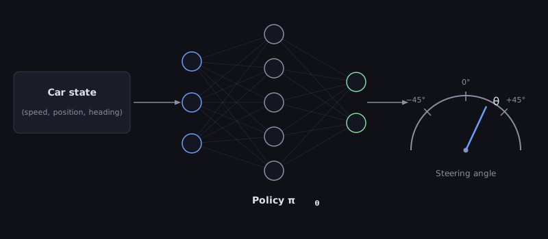
Now suppose we want to train a policy to estimate steering angle for a self-driving car.

Steering policy

Attempt 1: Predict a Single Value - A Deterministic Policy

The simplest approach: make the model output a single angle and train with L2 (MSE) loss.

The problem: mean-averaging. Imagine we collect data from four expert drivers, all in the same state:

Robot State	Expert Driver	Action (angle $\theta$)
s	Driver_1	-10°
s	Driver_2	+10°
s	Driver_3	-20°
s	Driver_4	+20°

With L2 loss, the model will learn to predict 0° — the mean of all expert actions.

Mean averaging problem

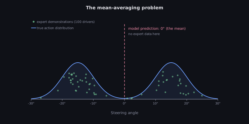
That’s neither left nor right, which could be catastrophic if the experts were, say, swerving to avoid an obstacle.

Beyond mean-averaging, deterministic policies have a compounding error problem

The model is trained on expert data, so it learns to predict well on states that the expert visits.
But at test time, if the model makes a small mistake and ends up in a state that the expert never visited, it has no idea what to do

Attempt 2: Predicting a Simple Distribution (Gaussian) - A Stochastic Policy

What if instead of predicting a single value, the model outputs the parameters of a Gaussian distribution — a mean $\mu$ and variance $\sigma^2$?

Gaussian policy

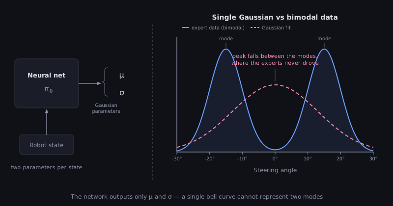
The expert data distribution for our steering example was bimodal (some drivers go left, some go right)
A single Gaussian can only capture one mode
If we train with L2 loss (which is equivalent to fitting the mean of a Gaussian), we again predict the average — right between the two modes.

Even if we somehow get the Gaussian to match one of the modes, we’re constraining the model to represent only a unimodal distribution. Not expressive enough.

Attempt 3: Gaussian Mixture Model - Slightly More Expressive Stochastic Policy

What if we ask the model to predict a mixture of Gaussians?

GMM policy

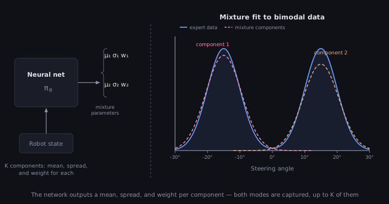
This is more expressive, but still limited by the number of mixture components we choose. If we pick 2 components, we can capture the bimodal distribution. But what if the expert data has 3 modes? Or 10 modes? We would need to arbitrarily choose a large number of components, which is inefficient and still may not capture the true distribution well.

Attempt 4: Autoregressive Models: Even More Expressive Stochastic Policies

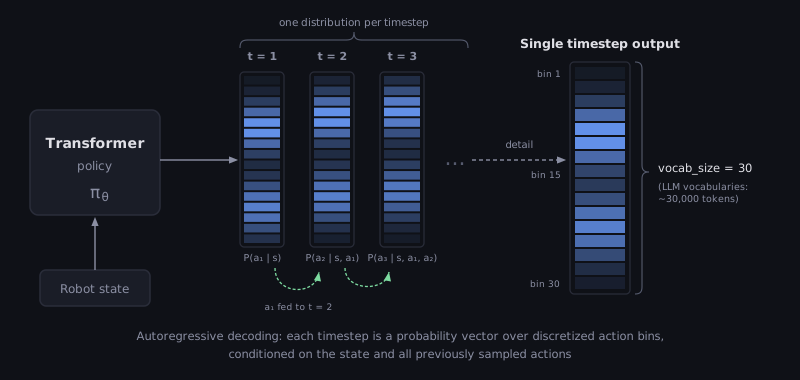
Transformer with timestep outputs

Here we rely on discretizing the action space into small enough ‘bins’ such that we are as ‘continous’ as possible. (our best approximation)

Bins to histogram

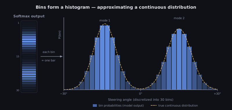
Each bin is again a probability (multi-class classification). More bins = more expressiveness, just like larger vocabulary size in LLMs.

Training Stochastic Policies with Maximum Likelihood

What does it actually mean to “match the expert”? The model outputs a probability distribution over actions. When the expert acts, we check: did our distribution put high probability where the expert acted? If yes, the loss is low. If not, the loss is high, and training shifts the distribution toward expert actions.

Extension: Predicting Multiple Actions per State

Autoregressive chain

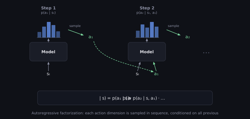
Attempt 5: Diffusion Policies — Most Expressive Continuous Stochastic Policies

Autoregressive models are maximally expressive but rely on discretizing the action space into bins. Diffusion policies keep actions continuous and still capture arbitrary multimodal distributions.

Quick recap: how diffusion works for images

In image generation (DDPMs, Stable Diffusion, etc.):

Take a clean image $x_0$, gradually corrupt it with Gaussian noise over $T$ steps until $x_T$ is pure noise.
Train a neural network to reverse that process — given a noisy image $x_t$ and the timestep $t$, predict the noise that was added.
At inference, start from random noise and iteratively denoise to produce a fresh image.

The output of the network is a noise prediction $\epsilon_\theta(x_t, t)$, and the loss is just MSE between predicted and actual noise. Conditioning (e.g., on a text prompt) is done by feeding it as an extra input to the network.

Now apply this to RL / behaviour cloning

In a diffusion policy, the “image” is the action and the “prompt” is the state.

Concretely, suppose the expert action $a_0 \in \mathbb{R}^d$ (e.g. $d=2$ for steering+throttle, or a 7-DoF arm joint vector). Then:

Training (one expert datapoint $(s, a_0)$):

Sample a random timestep $t \sim \mathrm{Uniform}{1, \dots, T}$.
Sample noise $\epsilon \sim \mathcal{N}(0, I)$ of the same shape as $a_0$.
Form a noisy action: $a_t = \sqrt{\bar\alpha_t}\, a_0 + \sqrt{1-\bar\alpha_t}\, \epsilon$. Here $\bar\alpha_t \in (0, 1)$ is a fixed schedule — as $t$ grows, $a_t$ looks more like pure noise.
Pass $(a_t, s, t)$ into the network. It outputs a noise prediction $\hat\epsilon = \epsilon_\theta(a_t, s, t)$.
Loss: $\lVert \epsilon - \hat\epsilon \rVert^2$. That’s it — a regression problem.

\[\mathcal{L}(\theta) = \mathbb{E}_{(s, a_0) \sim \mathcal{D},\, t,\, \epsilon}\!\left[\;\lVert \epsilon - \epsilon_\theta(a_t,\, s,\, t)\rVert^2\;\right]\]

The state $s$ is conditioning information — it’s fed in alongside $a_t$ and $t$, exactly the way a text prompt is fed into Stable Diffusion. The network learns to denoise toward actions that the expert would have taken in state $s$.

Inference (rolling out the policy in state $s$):

Sample $a_T \sim \mathcal{N}(0, I)$ — pure noise of shape $\mathbb{R}^d$.
For $t = T, T{-}1, \dots, 1$: query the network for $\hat\epsilon = \epsilon_\theta(a_t, s, t)$, then take a small step toward less noise:

\[a_{t-1} = \frac{1}{\sqrt{\alpha_t}}\!\left(a_t - \frac{1-\alpha_t}{\sqrt{1-\bar\alpha_t}}\, \hat\epsilon\right) + \sigma_t z, \quad z \sim \mathcal{N}(0, I)\]

After $T$ steps you have $a_0$, the action you actually execute on the robot.

So one “policy query” in state $s$ is $T$ forward passes through the denoising network — typically $T = 50$ to $100$, though faster variants (DDIM, consistency models) reduce this.

Why this is so expressive

The output of the policy is whatever distribution the iterative denoising lands you in. Each step is a small Gaussian update, but $T$ steps composed together can produce arbitrarily complex multimodal distributions over $a$. No bin discretization, no fixed mixture count.
Different initial noise samples $a_T$ naturally produce different modes. In the bimodal “swerve left or swerve right” example, half the noise samples denoise toward “left actions,” half toward “right actions” — the policy commits to one mode per query rather than averaging them. Mean-collapse is impossible by construction.
Action chunks are easy: instead of $a \in \mathbb{R}^d$, let the “image” be a sequence $(a_1, \dots, a_H) \in \mathbb{R}^{H \times d}$ of the next $H$ actions. The diffusion model denoises the whole chunk jointly, so multi-step plans stay temporally coherent. This is the setup in Chi et al.’s Diffusion Policy (2023).

Diffusion policies (e.g. Diffusion Policy by Chi et al., 2023) are state-of-the-art for many robotic manipulation tasks for exactly this reason — expert demonstrations are highly multimodal, and diffusion captures that without forcing a particular parametric form.

The trade-off: inference is slower (many denoising steps per action), though distillation and consistency models are actively shrinking that gap.

Summary: The Expressiveness Ladder

Approach	Output	Loss	Expressiveness
Deterministic	Single value	L2 (MSE)	Lowest — predicts the mean
Single Gaussian	$\mu, \sigma$	Gaussian NLL	Unimodal only
Mixture of Gaussians	$\{\mu_i, \sigma_i, w_i\}$	Mixture NLL	Multi-modal, fixed components
Autoregressive (discretized)	Bin probabilities	Cross-entropy	Maximally expressive (discrete)
Diffusion	Predicted noise $\epsilon_\theta$	MSE on noise	Maximally expressive (continuous)

The formal objective for expressive imitation learning:

\[\min_\theta \; -\mathbb{E}_{(\mathbf{s},\mathbf{a}) \sim \mathcal{D}}\left[\log \pi_\theta(\mathbf{a} \mid \mathbf{s})\right]\]

with an expressive distribution $\pi(\cdot \mid \mathbf{s})$. The more expressive the policy class, the better it can capture the full distribution of expert behavior.

Crafting Neural Nets for RL